from s1bursts import BurstCatalog, BurstProcessor, FileManager, SearchQuery, TimeRange

fm = FileManager("data/quickstart")
catalog = BurstCatalog(fm)

bursts = catalog.search(SearchQuery(
    time_range=TimeRange("2022-08-01", "2022-08-13"),
    burst_id=30346, sub_swath="IW1", polarization="VV",
))Quickstart
This example processes two acquisitions of one burst over the Aletsch glacier in the Swiss Alps. It produces terrain-corrected backscatter for each date and the coherence between them. Complete Installation first, and run the script with your credentials in the environment. The example downloads about 200 MB and runs SNAP.
Find two acquisitions
A search returns the catalog records that match a query. This one covers two weeks of one burst footprint, which Sentinel-1 imaged twice, 12 days apart:
Download and process
The download stores both acquisitions under data/quickstart/s1-slc. Processing then writes one GeoTIFF per product under data/quickstart/s1-prod. With crs="auto", each burst is projected in the UTM zone that holds it, here zone 32 North (EPSG:32632). Backscatter is processed per burst. Coherence needs a pair of acquisitions, which find_pairs() builds from the same bursts:
catalog.download(bursts).raise_on_failure()

processor = BurstProcessor(fm)
rtc = processor.create_backscatter(bursts, crs="auto").raise_on_failure()

pairs = bursts.find_pairs(baseline=12)
coherence = processor.create_coherences(pairs, crs="auto").raise_on_failure()
A burst that fails does not stop the others. raise_on_failure() raises an error naming every failed burst, and otherwise returns the summary of the run. Running the script again skips every file that already exists, after checking that it was made with the same settings.
Look at the result
Each product is a GeoTIFF that any GIS or raster library can open, and fm.open() opens one with rasterio. This plots the backscatter of the first date in decibels, with the coherence below it:
import matplotlib.pyplot as plt
import numpy as np

with fm.open(rtc.products[0]) as src:
    gamma0 = src.read(1, masked=True)
with fm.open(coherence.products[0]) as src:
    coh = src.read(1, masked=True)

fig, (top, bottom) = plt.subplots(2, 1, figsize=(7.8, 4.7), layout="constrained")
fig.colorbar(top.imshow(10 * np.log10(gamma0), cmap="viridis", vmin=-20, vmax=0),
             ax=top, label="Backscatter (dB)")
fig.colorbar(bottom.imshow(coh, cmap="magma", vmin=0, vmax=1), ax=bottom, label="Coherence")
for ax in (top, bottom):
    ax.set_axis_off()
plt.show()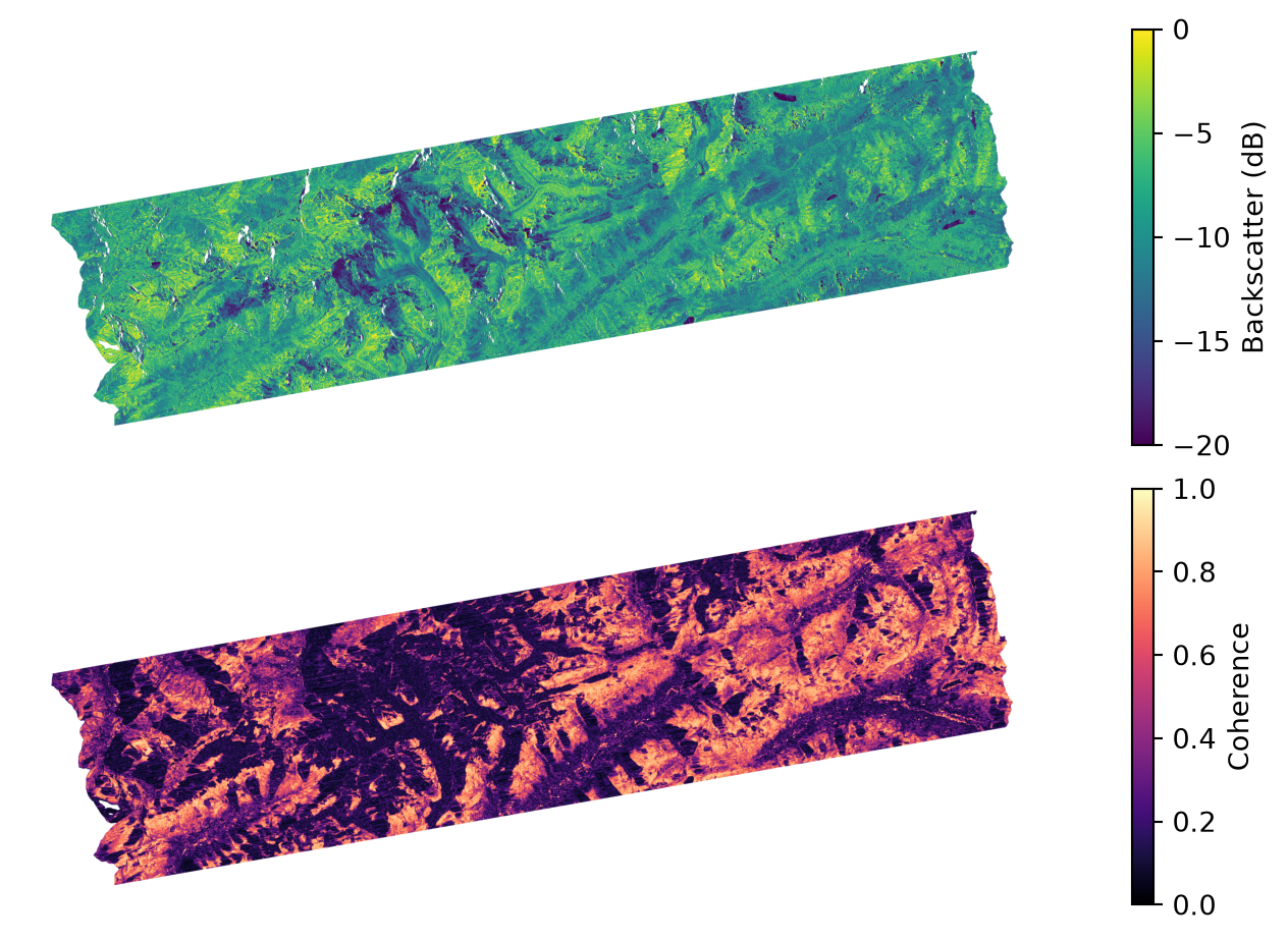
The burst covers a strip of the Alps about 85 km long. Coherence is high (light) where the ground changed little in the 12 days, such as bare rock and meadows, and low (dark) where it changed, for example on the melting glaciers and in forests.
What you get
The processing calls return two kinds of GeoTIFF:
- Backscatter (one file per date): how strongly the ground reflects the radar signal, corrected for terrain.
- Coherence (one file): how similar the two acquisitions are, from 0 (no similarity) to 1.
Products and bands explains each band and its units. The glacier tutorials take the same burst further.
NoteRun details
Run on 09 November 2026 with s1bursts 0.9.0 and ESA SNAP 13.0.0. Contains modified Copernicus Sentinel data (2022).