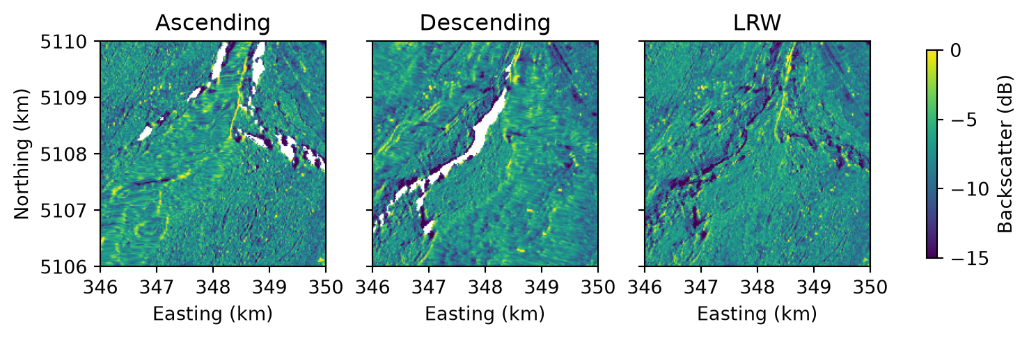
This tutorial runs the whole pipeline, from search to composites, for an area around Martigny in the Swiss canton of Valais. The town is surrounded by mountains, whose steep slopes are challenging terrain for SAR. The tutorial compares the single-pass composites, one of the ascending and one of the descending acquisitions, with a composite that combines both by local resolution weighting (LRW).
Find the bursts in the area of interest
The search finds the VV bursts that overlap the area’s grid square in a 12-day window, 2025-08-13 to 2025-08-24. The area lies in one 10 km square of the MGRS grid, and the search covers the entire square, as in From an area to composites:
from shapely.geometry import box
from s1bursts import (
    BurstCatalog, BurstProcessor, FileManager, MGRSGrid, ResolutionWeighter,
    RTCConfig, SearchQuery, TimeRange,
)

fm = FileManager("data/martigny")
catalog = BurstCatalog(fm)
aoi = box(7.01, 46.09, 7.055, 46.125)
window = TimeRange("2025-08-13", "2025-08-24")
(square,) = MGRSGrid(aoi, resolution=20)  # the area lies in one square
print(square.mgrs_code, square.crs)

search_area = box(*square.geographic_extent.boundingbox)
found = catalog.search(SearchQuery(time_range=window, intersects=search_area, polarization="VV"))
bursts = found.intersecting(square)

bursts.df.groupby(["pass_direction", "rel_orbit_number"]).agg(
    acquisitions=("date", lambda dates: dates.dt.date.nunique()),
    bursts=("burst_id", "size"),
    sub_swaths=("sub_swath", lambda names: ", ".join(sorted(names.unique()))),
    satellites=("parent_product_name", lambda names: ", ".join(sorted(names.str[:3].unique()))),
)
|
|
acquisitions |
bursts |
sub_swaths |
satellites |
| pass_direction |
rel_orbit_number |
|
|
|
|
| Ascending |
88 |
2 |
4 |
IW2 |
S1A, S1C |
| Descending |
66 |
2 |
4 |
IW3 |
S1A, S1C |
| 139 |
2 |
6 |
IW1, IW2 |
S1A, S1C |
One ascending and two descending orbits cover the square, each imaged twice in these 12 days, with 14 bursts in total.
Process backscatter
The bursts are processed in the UTM zone of the square, at 20 m grid spacing:
catalog.download(bursts).raise_on_failure()
processor = BurstProcessor(fm)
rtc = processor.create_backscatter(
    bursts, crs=square.crs, config=RTCConfig(grid_spacing=20),
).raise_on_failure().products
Compose the composites
To compare local resolution weighting with single-pass composites, the square is composed both ways. compose_rtc_lrw() combines both pass directions and also writes the quality layers, and compose_rtc_by_pass() averages each direction on its own, without weights. For an area of several squares, From an area to composites loops over them.
weighter = ResolutionWeighter(fm)
lrw = weighter.compose_rtc_lrw(rtc, square, write_qa=True, time_range=window)
by_pass = weighter.compose_rtc_by_pass(rtc, square, time_range=window)
Compare the composites
How finely a slope is resolved depends on how it faces the sensor. Sentinel-1 looks sideways, to the right of its track: east on ascending passes, west on descending ones. Slopes facing the sensor are compressed by foreshortening or layover and poorly resolved, while slopes facing away are well resolved or, if steep enough, fall into radar shadow, where that pass direction has no value (Why mountains need it).
import matplotlib.pyplot as plt
import numpy as np
from s1bursts.product import Layer


def read(composite, layer=Layer.MEASUREMENT):
    """Read one layer of a composite, with its extent in kilometers for imshow."""
    with fm.open(composite, layer) as src:
        left, bottom, right, top = (v / 1000 for v in src.bounds)
        return src.read(1).astype("float32"), [left, right, bottom, top]


view = (346, 350, 5106, 5110)  # easting and northing in km, UTM zone 32N
composites = {
    "Ascending": read(by_pass["Ascending"]),
    "Descending": read(by_pass["Descending"]),
    "LRW": read(lrw),
}
viridis = plt.get_cmap("viridis").copy()
viridis.set_bad("white")  # pixels without a value: radar shadow

fig, axes = plt.subplots(1, 3, figsize=(7.6, 3.2), sharey=True, layout="constrained")
for ax, (name, (data, extent)) in zip(axes, composites.items()):
    image = ax.imshow(10 * np.log10(data), extent=extent, cmap=viridis, vmin=-15, vmax=0)
    ax.set(title=name, xlabel="Easting (km)", xlim=view[:2], ylim=view[2:])
axes[0].set_ylabel("Northing (km)")
fig.colorbar(image, ax=axes, shrink=0.5, label="Backscatter (dB)")
plt.show()
Each single-pass composite has gaps where the steepest slopes facing away from the sensor fall into radar shadow, and compresses the slopes facing it into coarse streaks. The resolution-weighted composite averages all six acquisitions but gives the better-resolved ones more weight, so it has a value everywhere in this window, and its resolution varies less from slope to slope.
Check quality layers
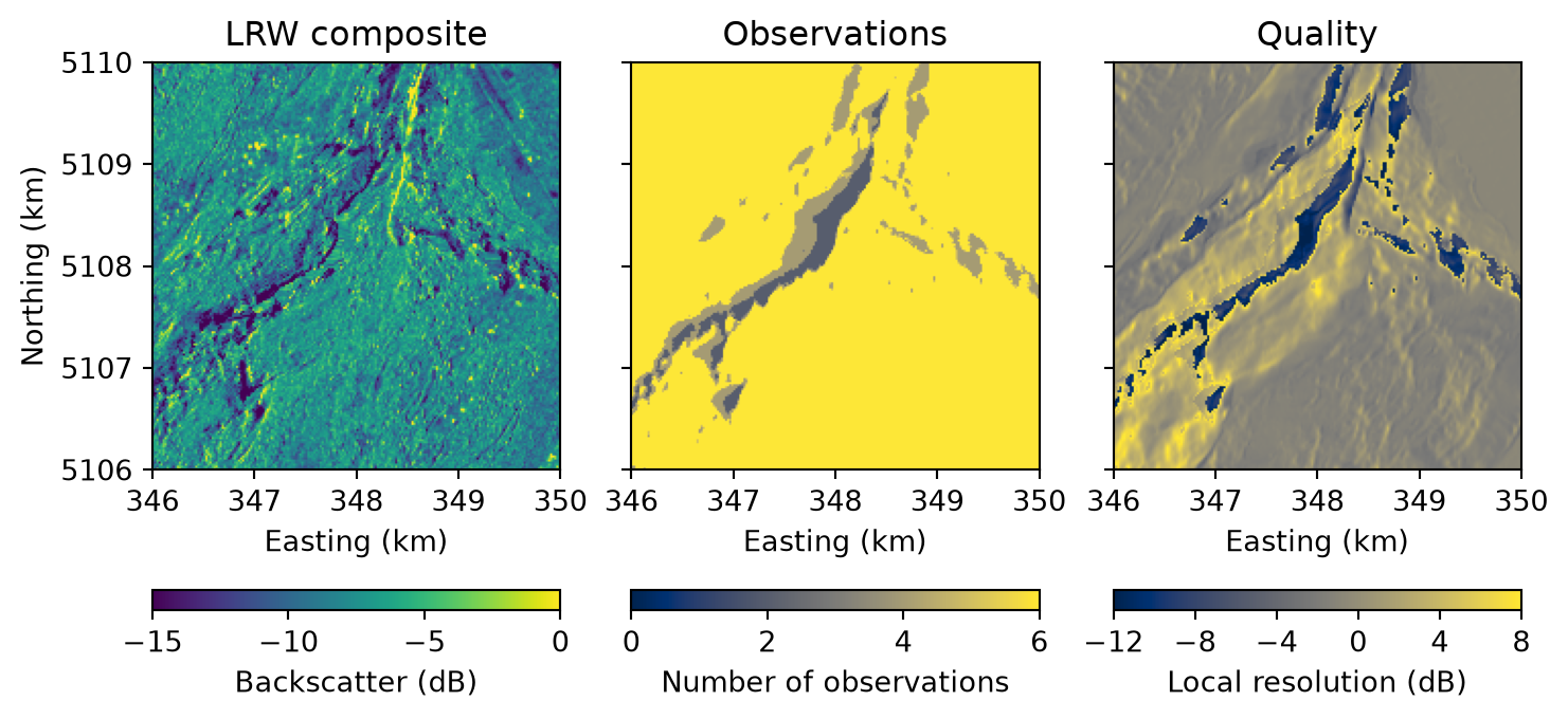
The LRW composite comes with two quality layers, shown here for the same window:
# title: (layer, colorbar label, colormap, colorbar ticks, the first and last being the limits)
layers = {
    "LRW composite": (Layer.MEASUREMENT, "Backscatter (dB)", "viridis", [-15, -10, -5, 0]),
    "Observations": (Layer.QA_NUM, "Number of observations", "cividis", [0, 2, 4, 6]),
    "Quality": (Layer.QA_CQM, "Local resolution (dB)", "cividis", [-12, -8, -4, 0, 4, 8]),
}
fig, axes = plt.subplots(1, 3, figsize=(7.6, 3.9), sharey=True, layout="constrained")
for ax, (title, (layer, label, cmap, ticks)) in zip(axes, layers.items()):
    data, extent = read(lrw, layer)
    if layer != Layer.QA_NUM:
        data = 10 * np.log10(data)
    image = ax.imshow(data, extent=extent, cmap=cmap, vmin=ticks[0], vmax=ticks[-1])
    fig.colorbar(image, ax=ax, orientation="horizontal", label=label, ticks=ticks)
    ax.set(title=title, xlabel="Easting (km)", xlim=view[:2], ylim=view[2:])
axes[0].set_ylabel("Northing (km)")
plt.show()
The number of observations (QA-NUM) counts the acquisitions outside radar shadow that contribute to each pixel: all six almost everywhere, fewer where one pass direction is in shadow. The composite quality map (QA-CQM) is the local resolution of the composite itself. It is highest on slopes that face away from the sensor in some orbits, and lowest on the steepest slopes, which every orbit either compresses or leaves in shadow. A pixel with a low quality describes the ground more coarsely than its 20 m grid spacing suggests. Local resolution weighting explains both layers.
Run on 09 November 2026 with s1bursts 0.9.0 and ESA SNAP 13.0.0. Contains modified Copernicus Sentinel data (2025).