from shapely import box

from freezebase.mgrs import MGRSGrid

aoi = box(5.8, 46.0, 6.5, 46.4)  # Geneva region; bare Shapely means WGS84 here
grid = MGRSGrid(aoi)

len(grid)48MGRSGrid provides reproducible 10 km raster targets for multi-source Earth Observation data. It is built on odc.geo: each square is a GeoBox carrying the CRS, affine transform, and array shape needed to place pixels on the ground.
A Sentinel-1 scene, a Sentinel-2 composite, a DEM, and a rasterised outline usually arrive in different projections, resolutions, and tiling schemes. If each new layer is aligned to whichever raster happens to be available first, the reference grid becomes an accidental property of the processing order.
MGRSGrid instead supplies a dataset-independent destination. For a given MGRS code and resolution, every pipeline derives the same CRS, transform, and shape. Sources resampled onto that destination are pixel-aligned by construction and can be stacked without another alignment decision.
The grid uses the Military Grid Reference System rather than inventing another spatial identifier:
It is established and metric. Each square lies on the metre-based lattice of a UTM zone. The grid is axis-aligned in its native projection, so a 10 m pixel represents a fixed 10 m grid spacing rather than a varying fraction of a degree.
Sentinel-2 uses the same reference system. A Sentinel-2 tile such as T32TMS corresponds to a 100 km MGRS square; a freezebase code such as 32TMS35 identifies one of its 10 km subdivisions. This makes the parent Sentinel-2 tile directly identifiable. Compatible 10 m data can be retiled without introducing an additional grid shift.
Ten kilometres is a practical unit of work. At 10 m resolution, a 100 km square contains 10,000 × 10,000 pixels, while a 10 km square contains 1,000 × 1,000. The smaller cells make it practical to download, cache, and process only the squares touched by scattered areas of interest.
Cells do not overlap within one UTM grid. Unlike Sentinel-2 product tiles, which include wasteful overlap around their 100 km reference squares1, freezebase cells step by exactly 10 km. Adjacent UTM zones are separate grids and can overlap; that limitation is described below.
Pass an area of interest in WGS84. The example deliberately crosses 6° E, the boundary between UTM zones 31 and 32:
from shapely import box
from freezebase.mgrs import MGRSGrid
aoi = box(5.8, 46.0, 6.5, 46.4) # Geneva region; bare Shapely means WGS84 here
grid = MGRSGrid(aoi)
len(grid)48to_geodataframe() returns one row per selected square in WGS84:
gdf = grid.to_geodataframe()
gdf.head()| mgrs_code | zone | hemisphere | easting | northing | epsg | geometry | |
|---|---|---|---|---|---|---|---|
| 0 | 31TGL19 | 31 | N | 710000 | 5090000 | 32631 | POLYGON ((5.83757 45.92833, 5.84216 46.01822, ... |
| 1 | 31TGL29 | 31 | N | 720000 | 5090000 | 32631 | POLYGON ((5.96638 45.92506, 5.97118 46.01494, ... |
| 2 | 31TGL39 | 31 | N | 730000 | 5090000 | 32631 | POLYGON ((6.09516 45.92164, 6.10018 46.01151, ... |
| 3 | 31TGM10 | 31 | N | 710000 | 5100000 | 32631 | POLYGON ((5.84216 46.01822, 5.84678 46.10811, ... |
| 4 | 31TGM11 | 31 | N | 710000 | 5110000 | 32631 | POLYGON ((5.84678 46.10811, 5.85143 46.198, 5.... |
The metadata includes the stable MGRS code, UTM zone and hemisphere, native EPSG code, and south-west corner in UTM metres. This AOI needs two local metric grids:
gdf.groupby(["zone", "epsg"]).size()zone epsg
31 32631 18
32 32632 30
dtype: int64GeoSeries or GeoDataFrame must declare WGS84 explicitly.resolution changes the pixels inside each selected square, not which squares are selected.Indexing or iterating over the grid yields MGRSGeoBox objects, a small subclass of odc.geo.geobox.GeoBox.
from odc.geo.geobox import GeoBox

square = grid[0]

display(square)
print(f"Is GeoBox: {isinstance(square, GeoBox)}")Is GeoBox: TrueIt combines image width, height, CRS, and an affine transformation to fully define a geo-registered pixel plane:
from odc.geo.geobox import GeoBox

square = grid[0]
print(f"mgrs_code:  {square.mgrs_code}")
print(f"crs:        {square.crs}")
print(f"shape:      {square.shape}")
print(f"resolution: {square.resolution}")
print(f"transform:\n{square.transform}")
print(f"is GeoBox:  {isinstance(square, GeoBox)}")
mgrs_code: 31TGL19
crs: EPSG:32631
shape: Shape2d(x=1000, y=1000)
resolution: Resolution(x=10, y=-10)
transform:
| 10.00, 0.00, 710000.00|
| 0.00,-10.00, 5100000.00|
| 0.00, 0.00, 1.00|
is GeoBox: TrueIt also brings along odc.geo operations and properties such as native and geographic extents.
Operations that derive a different box—such as padding, slicing, or reprojection—return a plain GeoBox. The derived box no longer has the exact footprint named by the MGRS code, so it intentionally does not retain mgrs_code.
When a code is already stored in a filename, database, or job description, the AOI does not need to be processed again:
from freezebase.mgrs import MGRSGeoBox, mgrs_to_crs

square = MGRSGeoBox.from_mgrs("32TMS35", resolution=10.0)
print(square)
print(mgrs_to_crs(square.mgrs_code))
MGRSGeoBox('32TMS35')
EPSG:32632This is why the grid is a specification rather than a dataset: the code and resolution are enough to reconstruct its georeferencing.
The resolution must be positive and divide 10 km evenly. Resolutions such as 10 m, 20 m, and 100 m therefore produce whole-pixel, nested grids with an integer scale factor:
for resolution in (10.0, 20.0, 100.0):
    cell = MGRSGeoBox.from_mgrs("32TMS35", resolution=resolution)
    print(f"{resolution:>5.0f} m -> {cell.shape}")
10 m -> Shape2d(x=1000, y=1000)
20 m -> Shape2d(x=500, y=500)
100 m -> Shape2d(x=100, y=100)freezebase implements the UTM portion of MGRS: 80° S to 84° N. It does not implement the polar UPS grids, so it does not cover every location on Earth.
Each UTM zone is projected independently. Cells within one zone share a non-overlapping 10 km lattice, but full cells retained along a zone edge can extend into the neighbouring zone. An AOI crossing that edge can consequently select cells from both zones that cover some of the same ground. This preserves coverage and keeps every cell square and axis-aligned in its own UTM CRS.
The structure is visible when the Geneva example is drawn in one display CRS:
import contextily as cx
import geopandas as gpd
import matplotlib.pyplot as plt
from matplotlib.patches import Patch
import pyproj

web_mercator = pyproj.CRS(3857)
squares = gdf.to_crs(web_mercator)
aoi_gdf = gpd.GeoDataFrame(geometry=[aoi], crs=4326).to_crs(web_mercator)
zone_colors = {31: "tab:blue", 32: "tab:red"}

fig, ax = plt.subplots(figsize=(9, 6))
for zone, color in zone_colors.items():
    squares[squares.zone == zone].plot(
        ax=ax, facecolor=color, alpha=0.25, edgecolor=color, linewidth=1.0
    )
aoi_gdf.boundary.plot(ax=ax, color="black", linewidth=2.0, linestyle="--")
cx.add_basemap(ax, source=cx.providers.CartoDB.Positron, crs=web_mercator, attribution_size=6)
ax.legend(
    handles=[
        *(
            Patch(facecolor=color, alpha=0.25, edgecolor=color, label=f"UTM zone {zone}")
            for zone, color in zone_colors.items()
        ),
        Patch(facecolor="none", edgecolor="black", linestyle="--", label="AOI"),
    ],
    loc="lower right",
)
ax.set_axis_off()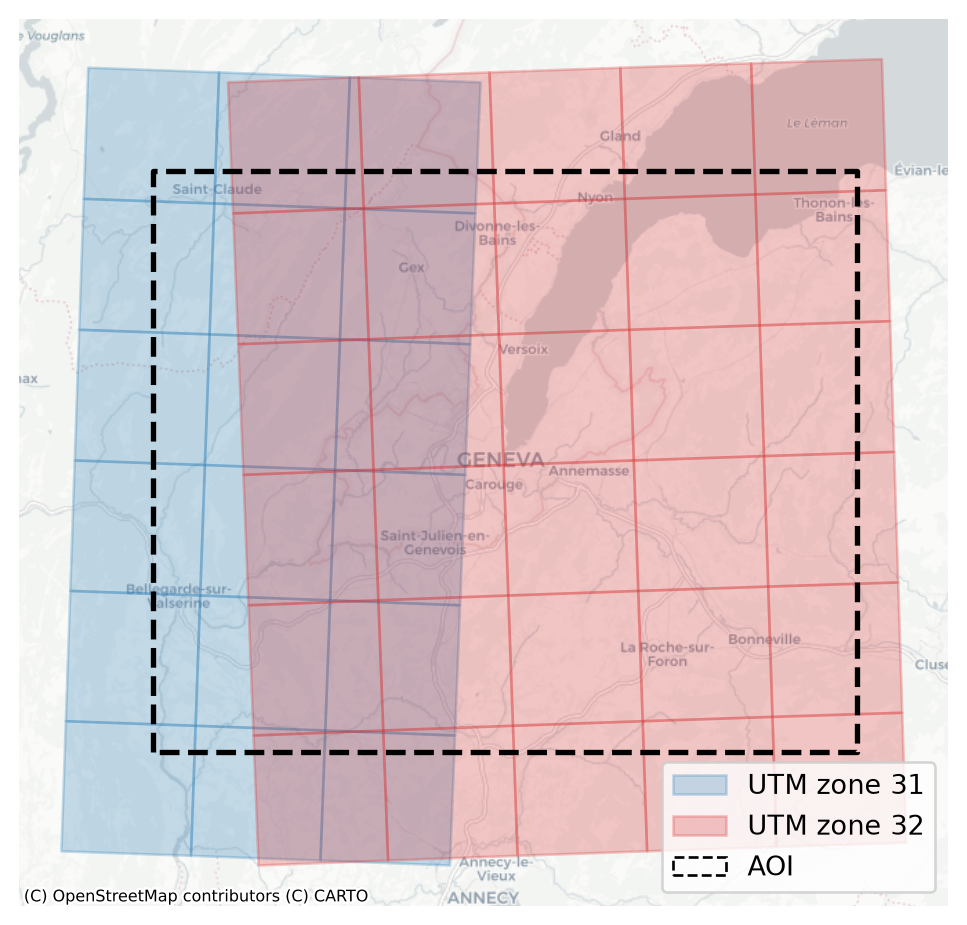
The Rasters on S3 guide shows how the same path abstraction can read a remote raster and resample it onto one of these boxes.
Bauer-Marschallinger, B., & Falkner, K. (2023). Wasting petabytes: A survey of the Sentinel-2 UTM tiling grid and its spatial overhead. ISPRS Journal of Photogrammetry and Remote Sensing, 202, 682–690. https://doi.org/10.1016/j.isprsjprs.2023.07.015↩︎