# Glacier backscatter time series

This tutorial follows the Aletsch glacier in the Swiss Alps through 2022, one acquisition per month. It shows how backscatter changes with the seasons and how to turn a stack of products into a time series for one site.


# Process one acquisition per month

The search covers a year of one burst footprint over the glacier. Keeping the first acquisition of each month leaves twelve, which are downloaded and processed into RTC backscatter at 20 m pixel size, in the burst's own UTM zone:


``` python
from s1bursts import BurstCatalog, BurstProcessor, FileManager, RTCConfig, SearchQuery, TimeRange
from s1bursts.burst import BurstCollection

fm = FileManager("data/glacier")
catalog = BurstCatalog(fm)
bursts = catalog.search(SearchQuery(
    time_range=TimeRange("2022-01-01", "2022-12-31"),
    burst_id=30346, sub_swath="IW1", polarization="VV",
))

df = bursts.df.sort_values("date")
monthly = BurstCollection(df.groupby(df.date.dt.month).head(1))
print(f"{len(bursts)} acquisitions in 2022, {len(monthly)} selected")
```


    30 acquisitions in 2022, 12 selected


``` python
catalog.download(monthly).raise_on_failure()
processor = BurstProcessor(fm)
rtc = processor.create_backscatter(
    monthly, crs="auto", config=RTCConfig(grid_spacing=20),
).raise_on_failure()
```


# Compare January and May

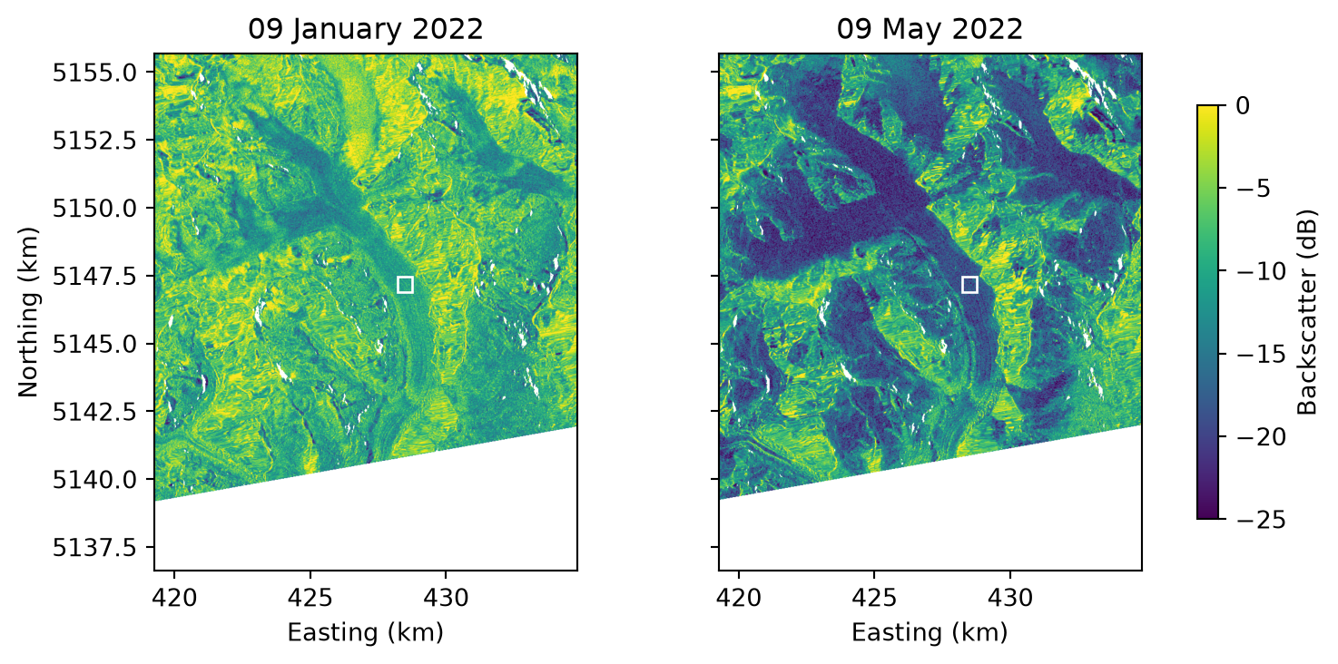
The maps show the glacier in January and in May. The tributaries of the Great Aletsch Glacier meet at Konkordiaplatz, near the top center, and the glacier flows south-east, then south-west toward its tongue. In May the glacier and much of the terrain around it are far darker than in January.


``` python
import matplotlib.pyplot as plt
import numpy as np
from rasterio.warp import transform_bounds
from rasterio.windows import from_bounds
from shapely.geometry import box

view = (7.95, 46.38, 8.15, 46.55)  # lon/lat bounds of the map
sample = box(8.065, 46.472, 8.072, 46.477)  # on the glacier below Konkordiaplatz
products = sorted(rtc.products, key=lambda p: p.date)

fig, axes = plt.subplots(1, 2, figsize=(7.8, 3.7), sharey=True, layout="constrained")
for ax, product in zip(axes, [products[0], products[4]]):
    with fm.open(product) as src:
        left, bottom, right, top = transform_bounds("EPSG:4326", src.crs, *view)
        gamma0 = src.read(1, window=from_bounds(left, bottom, right, top, src.transform))
        x0, y0, x1, y1 = transform_bounds("EPSG:4326", src.crs, *sample.bounds)
    extent = [v / 1000 for v in (left, right, bottom, top)]
    image = ax.imshow(10 * np.log10(gamma0), extent=extent, cmap="viridis", vmin=-25, vmax=0)
    ax.add_patch(plt.Rectangle((x0 / 1000, y0 / 1000), (x1 - x0) / 1000, (y1 - y0) / 1000,
                               fill=False, edgecolor="white"))
    ax.set(title=f"{product.date:%d %B %Y}", xlabel="Easting (km)")
axes[0].set_ylabel("Northing (km)")
fig.colorbar(image, ax=axes, shrink=0.8, label="Backscatter (dB)")
plt.show()
```


<figure class="figure">
<p><img src="glacier-backscatter_files/figure-html/cell-5-output-1.png" class="figure-img" width="737" height="366" /></p>
<figcaption>RTC backscatter around the Aletsch glacier in January and May 2022. The white rectangle is the sample area of the time series.</figcaption>
</figure>


# Extract a time series

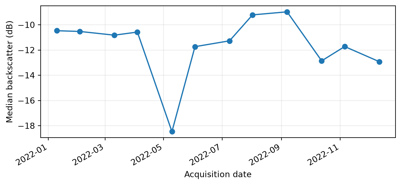
The time series is the median backscatter within the sample rectangle on the glacier. The median is taken in linear units and converted to decibels afterwards, because averaging decibels gives a biased result.


``` python
import pandas as pd
from rasterio.mask import mask
from rasterio.warp import transform_geom
from shapely.geometry import mapping

records = []
for product in products:
    with fm.open(product) as src:
        region = transform_geom("EPSG:4326", src.crs, mapping(sample))
        values, _ = mask(src, [region], indexes=1, crop=True, filled=False)
    valid = values.compressed()
    valid = valid[np.isfinite(valid)]
    records.append({"date": product.date, "gamma0_db": 10 * np.log10(np.median(valid))})
series = pd.DataFrame(records)
```


``` python
fig, ax = plt.subplots(figsize=(7.8, 3.3))
ax.plot(series.date, series.gamma0_db, "o-")
ax.set(xlabel="Acquisition date", ylabel="Median backscatter (dB)")
ax.grid(alpha=0.25)
fig.autofmt_xdate()
plt.show()
```


<figure class="figure">
<p><img src="glacier-backscatter_files/figure-html/cell-7-output-1.png" class="figure-img" width="656" height="303" /></p>
<figcaption>Median RTC backscatter in the sample rectangle, one acquisition per month in 2022.</figcaption>
</figure>


# Interpret the curve

Backscatter on the glacier stays near −10.5 dB from January to April, drops to −18.5 dB on 9 May, and recovers to about −9 dB in August and September. Wet snow is a likely cause of the drop: liquid water in the snowpack absorbs much of the radar signal, so wet snow appears dark (Rott, 1984)[^1]. From October, values settle around −12 to −13 dB.

The [next tutorial](glacier-coherence.md) computes coherence for the same burst.

> **Note: Run details**
>
> Run on 09 November 2026 with s1bursts 0.9.0 and ESA SNAP 13.0.0. Contains modified Copernicus Sentinel data (2022).


## Footnotes


[^1]: Rott, H. (1984). Synthetic aperture radar capabilities for snow and glacier monitoring. *Advances in Space Research*, 4(11), 241-246. <https://doi.org/10.1016/0273-1177(84)90418-6>